real-estate – Some Ben?

Going Out While Social Distancing

Wanna go to that kaiseki in The Mission? They have a 7 address, so our whole crew will be there.

My ‘rents just moved into the 123 High Street building. Now we can meet at the pub on the corner.

He does not stand a chance of a getting a star in Fam Three. The empty storefront next door is in Fam Five, though.

I expect us to be playing whack-a-mole with this pandemic for a few years, and am worried some indulgences of modern life will never come back. For example, fine dining is damn-near-impossible to do virtually. I have a background in the hospitality industry, and have had the privilege to eat some amazing meals in my life. So this is personal.

Now by fine dining, I mean the by-definition pretentious, wasteful, and amazing conversation between diner and chef via the medium of tiny bites on giant white plates. A prix fixe or à la carte menu enjoyed with wine & company over a few luxurious hours. Including the dreaded communal table thing too, I guess. But how are we going to eat at fancy restaurants while we continue to socially distance? And how are restaurant employees going to get back to making a (modest) living? Take-out fried chicken & cocktails from a Michelin star place desperate for cash flow just ain’t financially sustainable. Crenn is doing fancy comfort food like it’s October of 2001, but how is she going to pay rent in Russian Hill on $55 per head?

Lately a lot of my research is connecting a company’s stock price with the digital exhaust left when we interact with the world. A challenging part of the job is controlling for the bias in a cohort of people. When is a group actually representative of a population, or actually random? So while I am nothing close to a computational epidemiologist, and while every machine learning & data scientist is pretending to be a virus expert this week, I have one idea that might help with fine dining while we are in social isolation.

Take a Number for Going Out

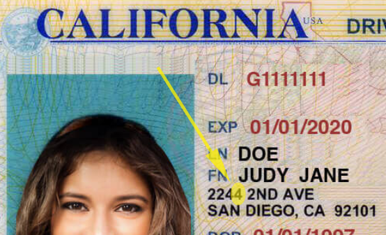
Imagine getting your driver’s license or passport checked at the entrance of a restaurant, where they confirm one simple fact: What is the last, right-most, least-significant digit of your mailing address? (Ignore fractions.) This digit is your membership in an slightly-different, in-real-life family — in which of ten virtual neighborhoods do you arbitrarily belong? And importantly, does your number match the last digit of the restaurant’s address? If the two IRL Fam numbers do not match, the restaurant would be mandated to refuse service. That’s it. Think through some implications of this simple restriction:

Maintains Social Isolation

When you go out to eat according to IRL Fam number, you are only ever physically near a fraction of the people in the world. And importantly, these people are always a semi-random subset of the same fraction of the population. The only people who are eating at the restaurant tonight are those who have the same number, those who are in the same IRL Fam. You might even get to know each other.

This is different from just going to local restaurants in the your zipcode, where a rando might jump a cab from across town for the restaurant’s particular charm. (This is especially relevant for experimental or avant garde places that have never relied on walk-ins.) The IRL Fam system is also fundamentally different from going to a different, random restaurant every weekend, because in this case you would still be exposed to a random set of people. And this is very different from restricting the number of people in a particular restaurant, simultaneously. A recent study from Cornell showed how even very small classes still would leave the student community highly connected. This would also thrash most restaurant’s finances.

What’s an address in 2020?

We could theoretically assign a random number, or use your mobile phone number, or even (shudder) use a Social Security number. However, there are additional benefits to using a physical, mailing address for layering our virtual spatial separation atop the existing physical world. Using your mailing address defaults a specific set of people into breaking your social distancing rules: Your roommates, family members, and those in your apartment building. Assuming you still like your kids & spouses after shelter-in-place eases, these are exactly the people you usually want to go out with. And these are the people from whom you are de facto not social distancing from, anyway! You share the same space, breath the same air, push the same elevators buttons, and so on.

What about the service?

This might require that restaurant employees only work full-time, and only at a single establishment. Would employees also need to have a matching IRL Fam? I think that would be too extreme, but goes in the right direction. Maybe we finally abandon the bullshit labor arbitrage of the gig economy, and pass a law establishing full-time de facto employment (i.e. benefits) for anyone who is works 40 hours a week for the same legal entity. San Francisco is already doing this with Uber drivers.

When’s your birthday?

This is no more a violation of privacy than when nightclub security checks the ID of your date who is looking particularly baby-faced tonight… Let’s mandate zero record-keeping or data retention on the IDs themselves, once the IRL Fam number is confirmed. I suppose patrons would need to have an ID with a mailing address on hand, which is a admittedly a bit classist.

Do they have valet parking?

Here is a significant downside. If you are not allowed in 90% of the restaurants in town, you are more likely to drive further to find an interesting one in your IRL Fam.

Is this all a game?

Given the prevalence of mostly-empty nightclubs with long lines, there is a chance the artificial exclusivity of the IRL Fam system would be fun and dramatic. An apartment with an address matching The New Hotness restaurant would be more desirable. And ironically, this exclusivity would be arbitrary and therefore, relatively fair!

Scaling & the Resurgence

This system could start in a traditionally-quirky place like San Francisco, and expand to restaurants & clubs & bars in other cities. And when the next pandemic (resurgence?) inevitably pops up, when the next shelter-in-place mandate occurs, contact tracing via IRL Fam number would be easier.

What is There to Eat Around Here?

Or, why clams are bourgeois — the presence of clams on menus is indicative of a place where people spend a lot of their money on housing. This is how I found out.

We have all played the proportional rent affordability game. How much of my income should I spend on where I live? One rule of thumb is “a third,” so if you take home $2,400 per month you aim to spend about $800 on rent or a mortgage payment. Some play the hypothetical budgeting version of the game. We might pay more of our income for housing if it means being able to live in a particularly desirable area.

Expensive Housing
Here is a map of income normalized by housing expense, for a bunch of Bay Area neighborhoods. This information is from our Altos Research active market real estate data. More technically, each dot on the map represents the ratio of a zipcode’s household income to the weighted average of single family home list prices and multi-family home list prices. I used median numbers, to minimize the impact of foreclosures or extremely wealthy households. Single and multi-family home prices were weighted by listing inventory, so urban condos matter as much as those McMansions in the ‘burbs. The green dots are areas where proportionally more income is spent on housing, and blue dots are the opposite.

The data shows that people living in the city of San Francisco spend a much larger proportion of their income on housing than Oaklanders or those in San Jose. If we assume that the real estate market is somewhat efficient, then those who choose to live in certain neighborhoods forgo savings and disposable income. Why is it that housing expenses for living in San Francisco are so much higher than San Jose, even when we control for income disparity?

The Real Estate Menu
Like a proper hack economist, I am going to gloss over the obvious driving factors of proportionally expensive housing, such as poor labor mobility, lack of job opportunities, and a history of minority disenfranchisement. I am a chef by training — culinary arts degree from CHIC, the Le Cordon Bleu school in Chicago — and remain fascinated by the hospitality industry. So instead of diving into big social problems, I focused on something flippant and easy to measure: Where people go out to eat, across areas with different levels of proportional housing expense.

I analyzed the menus of a random selection of 5,400 sit-down and so-called “fast casual” restaurants across the United States. This menu population is hopefully large and diverse enough to represent dining out in general, though it is obviously biased toward those restaurants with the money and gumption to post their menus online. However there is not a disproportionate number of national chain restaurants, since even the most common restaurant, T.G.I. Friday’s, is only about 2.5% of the population:

Menu Words
The next step in my analysis was counting the common words and phrases across the menus. Here are the top fifty:

1. sauce, 2. chicken, 3. cheese, 4. salad, 5. grilled, 6. served, 7. fresh, 8. tomato, 9. shrimp, 10. roasted, 11. served-with, 12. garlic, 13. cream, 14. red, 15. fried, 16. onions, 17. tomatoes, 18. beef, 19. rice, 20. onion, 21. bacon, 22. topped, 23. mushrooms, 24. topped-with, 25. steak, 26. vinaigrette, 27. spinach, 28. lettuce, 29. pork, 30. green, 31. potatoes, 32. spicy, 33. white, 34. salmon, 35. in-a, 36. soup, 37. peppers, 38. mozzarella, 39. lemon, 40. sweet, 41. with-a, 42. menu, 43. beans, 44. dressing, 45. fries, 46. tuna, 47. black, 48. greens, 49. chocolate, 50. basil

Pervasive ingredients like “chicken” turn up, as do common preparation and plating terms like “sauce” and “topped-with”. Perhaps my next project will be looking at how this list changes over time. For example, words like “fried” were taboo in the 90’s, but more common during this post-9/11 renaissance of honest comfort food. Now-a-days chicken can be “fried” again, not necessarily “crispy” or “crunchy”.

A Tasty Model
Next I trained a statistical model using the menu words and phrases as independent variables. My dependent variable was the proportional housing expense in the restaurant’s zipcode. The model was not meant to be predictive per se, but instead to identify the characteristics of restaurant menus in more desirable areas. The model covers over five thousand restaurants, so menu idiosyncrasy and anecdote should average out. The algorithm used was our bespoke version of least-angle regression with the lasso modification. It trains well on even hundreds of independent variables, and highlights which are most informative. In this case, which of our many menu words and phrases are correlated with proportional housing expense?

The twenty menu words and phrases most correlated with low proportional housing expense (the bluer dots) areas:

1. tortilla, 2. cream-sauce, 3. red-onion, 4. thai, 5. your-choice, 6. jumbo, 7. crisp, 8. sauce-and, 9. salads, 10. oz, 11. italian, 12. crusted, 13. stuffed, 14. marinara, 15. broccoli, 16. egg, 17. scallops, 18. roast, 19. lemon, 20. bean

Several of these words of phrases are associated with ethnic cuisines (i.e. “thai” and “tortilla”), and others emphasize portion size (i.e. “jumbo” and “oz” for ounce). Restaurants in high proportional housing expense areas (greener dots) tend to include the following words and phrases on their menus:

1. clams, 2. con, 3. organic, 4. mango, 5. tofu, 6. spices, 7. eggplant, 8. tomato-sauce, 9. cooked, 10. artichoke, 11. eggs, 12. toast, 13. roll, 14. day, 15. french-fries, 16. duck, 17. seasonal, 18. oil, 19. steamed, 20. lunch, 21. chips, 22. salsa, 23. baby, 24. arugula, 25. red, 26. braised, 27. grilled, 28. chocolate, 29. avocado, 30. dressing

These words reflect healthier or more expensive food preparation (i.e. “grilled” or “steamed”), as well as more exotic ingredients (i.e. “mango” and “clams”). Also, seasonal and organic menus are associated with low proportional housing expense. The word “con” turns up as a counter-example for Latin American cuisine, as in “con huevos” or “chili con queso”.

Food Crystal Ball
This sort of model for restaurant menus could also be used for forecasting, to statistically predict the sort of food that will be more successful in a particular neighborhood. This predictive power would be bolstered by the fact that the population of menus has a survivorship bias, because failed or struggling restaurants are less likely to post their menus online.

This confirms my suspicion that housing expense is counter-intuitive when it comes to dining out. People who spend more of their income on housing in order to live in a desirable location have less disposable income, but these are the people who pay more for exotic ingredients and more expensive food preparation. Maybe these folks can’t afford to eat in their own neighborhood?

Redots

Dorkbot is a semi-monthly meeting of “people doing strange things with electricity.” They have been chugging along in several cities for a decade-or-so. Back in 2005 I presented at a Dorkbot in London, so I have an enduring soft spot for these quirky gatherings. At this month’s Dorkbot in San Francisco, a meteorologist named Tim Dye presented a brilliant visualization called WeatherDots. It summarizes the weather data he collects near his home in wine country.

Inspired by how much time-series information Dye was able to squeeze onto a few pretty circles, I spent the plane ride to ABS East in Miami throwing together a “dot” visualization of the Altos Research weekly active market data. Here is a visualization of a year’s worth of real estate data:

http://www.altosresearch.com/customer/labs/redots.html

My Redots updates every week, and can be pointed at any of the Altos Research local markets by entering a city, state, and zipcode. Your web browser needs to play nicely with the amazing Raphaël visualization library, or you will just get a blank screen. I recommend using Google Chrome.

The Legend, or What Is It?
Each dot of color represents a week in a local residential real estate market, so each column is a month. The main color of the dot shows the week-on-week change in the median price of single family homes in a particular zipcode. A red dot means house prices have decreased since the previous week (or dot), while green dots are increasing weeks. The summer seasonality effect is pretty clear in our Mountain View, CA example.

The “halo” of a dot is the ratio of new listings to listings in general. If the newest listings coming onto a market are priced higher than the typical listing, then the halo will be green. This suggests a seller’s market, when new listings are asking for a premium. The price of these new listings will be absorbed into the market the following week, so you might imagine a dot’s halo merging with the main color.

A dot’s angle is the year-on-year change in market prices. Aiming northeastward means prices have increased since the year before, while southeast is a decrease. These angles strip away seasonality from the market, and show how secular real estate trends. Our Silicon Valley example is a bit down year-on-year. The thickness of a weekly dot represents the week-on-week change in the number of listings, put more simply, the inventory. Thin dots that are more ellipsoid are a shrinking market, where fewer listings are available for sale at any price.

A Thousand Words
Information visualization is a buzzy field with smart people doing striking work. For me the line between the big data and infovis communities blurs when a pretty picture enables statistical inference without necessarily running the numbers.

A Different House Hedge

Where do stock market winners buy houses?

There are many ways to predict how the price of an asset will change in the future. For stocks, one approach is based on fundamental analysis and another approach uses portfolio diversification theory. A third approach to predicting stock movement is so-called “technical analysis,” which is too silly for more than a mention. There are also statistical arbitrageurs in the high-frequency market-making and trading arms race, who make minute predictions thousands of times per day. If we pretend real estate acts as a stock, we can stretch the analogy into a new mathematical tool for hedging house prices.

Fundamentalism

Fundamental analysis is usually what people think about when picking stocks. This is the Benjamin Graham philosophy of digging into a company’s internals and financial statements, and then guessing whether or not the current stock price is correct. The successful stock picker can also profit from an overpriced share by temporarily borrowing the stock, selling it, and then later buying it back on the cheap. This is your classic “short,” which may or may not be unethical depending on your politics. Do short trades profit from misery, or reallocate wasted capital?

Fundamental analysis is notoriously difficult and time-consuming, yet it is the most obvious way to make money in the stock market. Fundamental analysis is also what private equity and venture capitalists do, but perhaps covering an unlisted company or even two guys in a garage in Menlo Park. When you overhear bankers talking about a “long/short equity fund” they probably mean fundamental analysis done across many stocks and then managing (trading) a portfolio that is short one dollar for every dollar it is long. This gives some insulation against moves in a whole sector, or even moves in the overall economy. If you are long $100 of Chevron and short $100 of BP, the discovery of cheap cold fusion will not trash your portfolio since that BP short will do quite well. However for conservative investors like insurance companies and pension funds, government policy restricts how much capital can be used to sell assets short. These investors are less concerned about fundamental analysis, and more about portfolio diversification and the business cycle.

Highly Sensitive Stuff

If a long-only fund holds just automobile company stocks, the fund should be very concerned about the automobile sector failing as a whole. The fund is toast if the world stops driving, even if their money is invested in the slickest, most profitable car companies today. Perfect diversification could occur if an investor bought a small stake in every asset in the world. Though huge international indices try to get close, with so many illiquid assets around, perfect diversification remains just a theory. How can an investor buy a small piece of every condominium in the world? How could I buy a slice of a brand like Starbucks? Even worse, as time goes by companies recognize more types of illiquid assets on their balance sheets. Modern companies value intellectual property and human capital, but these assets are difficult to measure and highly illiquid. What currently unaccounted-for asset will turn up on balance sheets in 2050?

Smart fund managers understand that perfect diversification is impossible, and so they think in terms of a benchmark. A fund benchmark is usually a published blend of asset prices, like MSCI’s agricultural indices. The fund manager’s clients may not even want broad diversification, and may be happy to pay fund management fees for partial diversification across a single industry or country. Thinking back to our auto sector fund, they are concerned with how the fortune’s of one car company are impacted by the automobile industry as a whole. An edgy upstart like Tesla Motors is more sensitive to the automobile industry than a stalwart like Ford, which does more tangential business like auto loans and servicing.

Mathematically we calculate the sensitivity of a company to a benchmark by running a simple linear regression of historic stock returns against changes in the benchmark. If a company’s sensitivity to the benchmark is 2.5, then a $10 stock will increase to $12.50 when the benchmark goes up by one point. A sensitivity of 0.25 means the stock would just edge up to $10.25 in the same scenario. A company can have negative sensitivity, especially against a benchmark in another related industry. Tesla probably has a negative sensitivity to changes in an electricity price index, since more expensive electricity would hurt Tesla’s business. No sensitivity (zero) would turn up against a totally unrelated benchmark. Sensitivity has a lot in common with correlation, another mathematical measure of co-movement.

One type of sensitivity is talked about more than any other. “Beta” is the sensitivity of a stock to the theoretical benchmark containing every asset in the world. Data providers like Bloomberg and Reuters probably estimate beta by regressing stock returns against one of those huge, international asset indices. An important model in finance and economics is called the Capital Asset Pricing Model, which earned a Nobel Prize for theorizing that higher beta means higher returns, since sensitivity to the world portfolio is the only sort of risk that cannot be diversified away. Though the CAPM beta is a poor model for real-life inefficient markets, sensitivities in general are a simple way to think about how a portfolio behaves over time. For instance, it turns out that sensitivities are additive. So $100 in a 0.25 sensitive stock and $50 in two different -0.25 sensitive stocks should be hedged against moves in the index and in the industry the index measures.

Back to Real Estate

Prices in certain local real estate markets are bolstered by a rally in the stock market. The recent murmurings of another IPO bubble suggest that newly minted paper millionaires will soon be shopping for homes in Los Altos Hills and Cupertino. We can put numbers behind this story by calculating real estate price sensitivity to a stock market benchmark. If we choose the S&P 500 as the benchmark, the sensitivity number will be a sort of real estate beta. Since real estate is far less liquid than most stocks, I regressed quarterly changes in our Altos Research median ask price against the previous quarter’s change in the S&P 500. Historically speaking, those real estate markets with a high beta have gotten a boost in prices after a good quarter in the stock market. Those markets with a low, negative beta are not “immune” to the stock market, but tend to be depressed by a stock market rally.

Below is a map of the Bay Area’s real estate betas. These numbers were calculated using prices from Altos Research and benchmark levels from Yahoo! Finance. The darker red a zipcode, the greater an increase in the market’s home prices after a quarterly stock market rally. As we might expect, the betas in Silicon Valley are above average. However there are also some surprises in Visalia and Wine Country.

Our hypothesis for positive real estate beta is easy: those IPO millionaires. But what could cause a real estate market to tank after a good run in the stocks? Perhaps negative real estate betas are in more mobile labor markets, where stock market wealth triggers a move away from home ownership. Or maybe negative real estate betas turn up in markets where the condo stock is higher quality than single-family homes, like in some college towns. Remember the betas mapped above are based on only single-family home prices.

Real estate remains a difficult asset to hedge, an asset almost impossible to short by non-institutions. This is unfortunate, because a short hedge would be a convenient way for people with their wealth tied up in real estate to ride out a depressed market cycle. However like long-only fund managers, real estate investors could benefit from thinking in terms of benchmark sensitivity. If we choose a benchmark that represents the broader real estate market, we could hedge real estate buy purchasing non-property assets that have negative real estate betas. You would want your value-weighted real estate beta to net out to about zero. Now there is a plethora of problems and assumptions around making investment decisions with a crude linear sensitivity number, but at least real estate beta gives us another tool for thinking about housing risk.

(An abbreviated version of this post can found be at http://blog.altosresearch.com/a-different-house-hedge/ on Altos Research’s blog)

Fungal Houses

Ever wondered why your flat’s Zestimate bounces around so much?

In high school economics class you might have learned about fungible goods. This strange word refers to things that could be swapped without the owners especially caring. A dollar is almost perfectly fungible, and so is an ounce of pure silver. Paintings and emotional knick knacks are not at all fungible. Fungible stuff is easy to trade on a centralized market, since a buyer should be happy to deal with any seller. This network effect is so important that markets “push back,” and invent protocols to force fungibility. Two arbitrary flatbeds of lumber at Home Depot are probably not worth the same amount of cash. However the CME’s random length lumber contract puts strict guidelines on how that lumber could be delivered to satisfy the obligation of the future contract’s short trader.

Real estate is seriously non-fungible. Even a sterile McMansion in the suburbs can have a leaky roof, quirky kitchen improvements, or emotional value for the house-hunting recent college grads. If we consider many similar homes as a basket, or a portfolio of the loans secured by the homes, then the idiosyncrasies of each home should net out to zero overall. Across those ten thousand McMansions, there should be a few people willing to pay extra for a man cave, but also a few people who would dock the price. This is the foundation of real estate “structured products,” such as the residential mortgage backed securities (RMBS) of recent infamy. Like flatbed trucks delivering a certain sort of wood for a lumber futures contract, a RMBS makes a non-fungible good more fungible.

The Usual Place
The combined idiosyncrasies of non-fungible things rarely net out to exactly zero, especially during a financial crisis. Nonetheless traders and real estate professionals want to think about a hypothetical, “typical” property. We define a local real estate market by city, neighborhood or even zipcode. How do we decide the value of a typical property? There is an entire industry built around answering this question. One simple, clean approach is to sample a bunch of real estate prices in a local market at a certain point in time, and then average the prices. Or maybe use a more robust descriptive statistic like the median price.

The most readily available residential home prices in the U.S. market are “closed” transactions, the price a home buyer actually paid for their new place. Using a closed transaction price is tricky, because it is published several months after a property is sold. Can a typical home price really be representative if it is so stale?

Sampling
Even if we ignore the time lag problem, there is another serious challenge in using transactions to calculate a typical home price. Within any local real estate market worth thinking about, there are very few actual transactions compared with overall listing activity and buzz. Your town may have a hundred single-family-homes listed for sale last week, but only four or five closed purchases. A surprise during the buyer’s final walkthrough could wildly swing the average, “typical” home price. For the statistically inclined, this is a classic sample size problem.

There are plenty of ways to address the sample size problem, such as rolling averages and dropping outliers. Or you could just include transactions from a wider area like the county or state. However the wider the net you cast, the less “typical” the price!

Another approach is to sample from the active real estate market, those properties currently listed for sale. You get an order of magnitude more data and the sample size problem goes away. However everyone knows that listing prices do not have a clear cut relationship with closing price. Some sellers are unrealistic and ask too much, and some ask for too little to start a bidding war. What is the premium or discount between listing price and actual value? We spend a lot of time thinking about this question. Even closed transaction prices are not necessarily the perfect measure of typical “value” since taxes and mortgage specifics can distort the final price. Our solution is to assume that proportional changes in listing prices over time will roughly match proportional changes in the value of a typical house, especially given a larger sample from the active market.

A Picture
Below is a chart of Altos Research‘s real estate prices back through 2009, across about 730 zipcodes. For each week on the horizontal axis, and for each zipcode, I calculate the proportional change in listing price (blue) and in sold price (red) since the previous week. Then I average the absolute value of these proportional changes, for a rough estimate of volatility. The volatility of sold prices is extreme.

Case-Shiller April Forecasts

Another finger in the air, in the beginning of the month lull.

My forecasts for the March, 2011 Case-Shiller index levels were quite rushed. They were released quickly so I could publicly compare the forecasts with the CFE futures contracts about to expire. However, since the statistical models use active market data, there is no mathematical reason to wait on our forecasts until the end of the month. The April, 2011 index levels will be released on June 28th, but here are my forecasts given what the real estate markets were doing a few months ago:

City	Confidence	Forecast	Predicted HPI
Minneapolis, MN	+1	-10.52%	94.46
Phoenix, AZ	+1	-2.85%	97.42
Las Vegas, NV	+3	-1.56%	95.67
Atlanta, GA	+2	-1.45%	96.93
Boston, MA	0	-1.32%	145.42
Los Angeles, CA	-2	-1.22%	165.73
Seattle, WA	+3	-0.46%	132.35
New York, NY	-1	-0.21%	163.15
San Francisco, CA	-3	-0.20%	129.56
Chicago, IL	+2	-0.06%	110.50
San Diego, CA	-3	+0.18%	154.16
Detroit, MI	0	+0.41%	67.34
Charlotte, NC	0	+0.50%	107.50
Miami, FL	0	+1.01%	138.66
Dallas, TX	+1	+1.62%	114.72
Cleveland, OH	+1	+2.12%	98.85
Denver, CO	0	+2.27%	123.29
Tampa, FL	+1	+2.28%	129.98
Portland, OR	+1	+4.71%	138.92
(The confidence score ranges from negative three for our weakest signals, up to positive three for strength. Unfortunately I am still sorting out a bug in our Washington, DC model.)

Housing Finger in the Air

The March, 2011 Case-Shiller numbers will be released this Tuesday, but the CME’s May futures contracts expire tomorrow. Some of the real estate transactions that will be summarized in Tuesday’s numbers are up to five months old, where our data is at most one week old. This is why Altos Research calls its statistics “real time,” since it is an order of magnitude more current than the benchmark in real estate data.

Below is a table of our forecasts for six of the Case-Shiller futures contracts. Check back in a few days, when I will compare with the actual March, 2011 numbers.

Metro Area	Feb-2011 CS HPI	Forecast	Signal
Boston, MA	149.86	-2.33%	111bps below the future’s spot bid price
Chicago, IL	113.26	-1.28%	in the spread
Denver, CO	121.26	-3.31%	64bps below the future’s spot bid price
Las Vegas, NV	98.28	-3.26%	96bps below the future’s spot bid price
Los Angeles, CA	168.25	-8.64%	763bps below the future’s spot bid price
San Diego, CA	155.05	+1.66%	209bps above the futures spot ask price
(all spot prices as of 10:30am PST on 26-May-2011)

Fighting the Last War: Shiller Paper

A new type of mortgage gets a price that means you never have to walk away.

Last month Robert J. Shiller, Rafal M. Wojakowski, Muhammed Shahid Ebrahim and Mark B. Shackleton published a paper with the financial engineering to price “continuous workout mortgages.” This is the Shiller of Irrational Exuberance and housing index fame.

A continuous workout mortgage leaves some of the risk of house price deprecation with the mortgage lender, since the mortgage balance automatically adjusts if the market tanks. The authors model an interest-only continuous workout mortgage as a loan bundled with a put option on the value of the home and a floor on interest rates. By design, the option to abandon the mortgage is always out of the money, so the borrower has little incentive to strategically default or walk away.

Pricing a continuous workout mortgage uses a standardized housing index. Perversely, this prevents a borrowers from trashing their own homes in order to reduce payments. So the bundled put option is on a housing index and not on the exact home. Others have written about the political and class bias encouraged when your savings are connected so directly to the neighborhood. Standard & Poor’s conveniently sells metropolitan housing indices. These S&P Case-Shiller housing indices have serious problems, including methodology transparency and data lag — no one can replicate and therefore validate the Case-Shiller numbers, the indices are published several months late, and they ignore the prices of homes pulled off the market without a sale.

Like proper quants, Shiller and colleagues push hard for a closed-form pricing formula. The party line is that clean formulas make for better markets, but computer simulation is easy enough now-a-days and far more accurate. Ahh, job security! To get a formula for the interest rate a lender should charge for a continuous workout mortgage, they make the heroic Black-Scholes universe assumptions, including:

The housing index can be traded, and traded without any brokerage fees. Also the index can be sold or bought for the same price.
Cash can be borrowed or lent at the exact same interest rate.
No one pays taxes.
The variance (jitter) in the housing index is independent of how much a trader expects to earn from investing in the housing index. This one is rarely mentioned, but not so obscure once you drop the “risk neutral” jargon.

And so also like proper quants, Shiller and his colleagues assume the frictionless, massless pulley from a high school physics class.