Dumpster Language

NLP analysis done on a dataset of about 8,000 transcripts of Dumpster (as in “Trump’s a Dumpster-fire”) back to 2007. Unfortunately there are no trends that obviously jump out. He has probably been keeping to book more closely than generally expected, at least in these prepared interviews.

Here are three early transcripts: “xx00133” from Showbiz Tonight (CNN in 2006), “xx00598” from Your World with Neil Cavuto (Fox in 2009), and “xx00911” from Nightline (ABC in 2009):

How has the implied grade-level and complexity of Dumpster’s speaking changed over time?

How has his information content changed over time (empirical bag-of-words entropy)?

If I assume the distant past is the benchmark for Dumpster authorship, does the recent speaker seems like the same person? (This is function word distribution.)

Happy Birthday, Hipsteraunt

Last month was the two year anniversary of the website Hipsteraunt, which I built with my friend Lance Arthur. He did the design, I did the random menu generation. It is a quirky bit of AI and NLP under-the-hood, so a user gets menus featuring free-range suspended chicken feet, truffled shisito pepper with achiote, and marshmallow crudo, at a place with an ampersand in its name. The inspiration had been a particular dinner out in San Francisco, at an immensely overrated restaurant. But it could have been Brooklyn or the West Loop. I am a quant & machine learning researcher by happy vocation, but also a chef by training. (Le Cordon Bleu with honors, thank you.) So the term “foodie” has always struck me as what privileged folks call themselves when they like to eat fancy food, but would not be caught dead hanging out with a line cook.

Hipsteraunt remains a tender satire of a certain sort of fetishized dining out. It was meant to be an acerbic call to check-your-privilege, together with a reminder that nothing in food is new. No combination of ingredients or flavors has not been tried a thousand times before. Even offal and the Asian flavors everyone loves to exoticize. (Awkward…) We lived through the fusion cuisine of the 1980s, remember? In hindsight, it might have cut a bit too close to the bone. The site garnered plenty of attention, but less heady pokes like the fake Guy Fieri menu and the brilliant Jacques le Merde have been far more successful. An annoying bug with making menu URLs permanent snagged things up the first couple weeks, too. Nonetheless on Hipsteraunt’s second birthday, I celebrate by raising an artisanal cocktail (a lemongrass aviation, perhaps) and toasting the addition of a few new ingredients: Keep an eye out for those trendy signifiers of faux-edgy cuisine we all love, like burrata and purslane, za’atar and togarashi. Goodbye ginger, goodbye almond milk. But it looks like bacon is still there.


Outside Ukulele

A model for the POU, probability -of- ukulele.

The Outside Lands 2014 lineup looks to be one of the best in years, and as usual it will be difficult to decide which stage to watch over the weekend. To help, I wrote an NLP model that measures the degree to which a band is likely to lapse into entitlement and self-parody. So think of it as a musical spectrum, from Kanye West to Death Cab for Cutie.

  1. Kanye West
  2. Flume
  3. Paolo Nutini
  4. Ben Howard
  5. Watsky
  6. Ray LaMontagne
  7. Duck Sauce
  8. Jonathan Wilson
  9. Run the Jewels
  10. Jagwar Ma
  11. Tiësto
  12. Big Freedia
  13. Lykke Li
  14. The Brothers Comatose
  15. Kacey Musgraves
  16. Valerie June
  17. Atmosphere
  18. Tycho
  19. Macklemore & Ryan Lewis
  20. Tom Petty & the Heartbreakers
  21. Tegan & Sara
  22. Haim
  23. Bleachers
  24. Holy Ghost!
  25. Christopher Owens
  26. Dum Dum Girls
  27. Lucius
  28. Gold Panda
  29. Courtney Barnett
  30. Vance Joy
  31. Bear Hands
  32. RayLand Baxter
  33. Gardens & Villa
  34. Imelda May
  35. Mikal Cronin
  36. Finish Ticket
  37. Tumbleweed Wanderers
  38. Boys Noize
  39. SBTRKT
  40. The Kooks
  41. The Flaming Lips
  42. The Killers
  43. Grouplove
  44. Warpaint
  45. Arctic Monkeys
  46. Chromeo
  47. Typhoon
  48. Chvrches
  49. Capital Cities
  50. Local Natives
  51. John Butler Trio
  52. Deer Tick
  53. Greensky Bluegrass
  54. Woods
  55. Tedeschi Trucks Band
  56. The Soul Rebels
  57. The Districts
  58. Nicki Bluhm and The Gramblers
  59. Spoon
  60. Jenny Lewis
  61. Phosphorescent
  62. Cut Copy
  63. Night Terrors of 1927
  64. Givers
  65. Disclosure
  66. Death Cab For Cutie

New Sentiment Dataset

The good folks in Stanford’s Natural Language Processing Group have built a powerful new dataset for a paper being presented at the EMNLP conference in Seattle next month. The underlying foundation of the dataset is not particularly exciting, being yet another corpus of labeled movie reviews: The review sentence “Stealing Harvard doesn’t care about cleverness, wit or any other kind of intelligent humor” is provided along with its negative sentiment label, for example. What is more interesting is the corpus providing sentiment labels at every level of composition. So for the same sentence, the dataset also provides a distinct sentiment label for the sub-phrase “any other kind of intelligent humor” which is actually positive. Hence the dataset is a treebank, not just your typical corpus. A lot of Mechanical Turk wrangling went into this! This compositional and recursive labeling is a great resource for training contextual models, especially ones that go beyond the bag-of-words legacy.

Here at Trending we are experimenting with an online, regularized, high-dimensional linear approximation to the Stanford paper’s tensor RNN model, one that lets us use the whole Vowpal Wabbit stack. Next month they plan to release some (Matlab) code to parse the treebank, but have already released the data itself. Therefore I put together a simple Ruby module to parse the treebank, for your own statistical NLP, sentiment and machine learning projects. It includes a bit of Graphviz logic to render phrase trees and their sentiment as SVG:

The module is hosted on Github at “http://github.com/someben/treebank/” under a nice Free license.

Hashing Language

How do you build a language model with a million dimensions?

The so-called “hashing trick” is a programming technique frequently used in statistical natural language processing for dimensionality reduction. The trick is so elegant and powerful that it would have warranted a Turing Award, if the first person to use the trick understood its power. John Langford cites a paper by George Forman & Evan Kirshenbaum from 2008 that uses the hashing trick, but it may have been discovered even earlier.[1] [2] Surprisingly most online tutorials and explanations of the hashing trick gloss over the main insights or get buried in notation. At the time of this writing, the Wikipedia entry on the hashing trick contains blatant errors.[3] Hence this post.

Hash, Man

A hash function is a programming routine that translates arbitrary data into a numeric representation. Hash functions are convenient, and useful for a variety of different purposes such as lookup tables (dictionaries) and cryptography, in addition to our hashing trick. An example of a (poor) hash function would map the letter “a” to 1, “b” to 2, “c” to 3 and so on, up to “z” being 26 — and then sum up the numbers represented by the letters. For the Benjamin Franklin quote “beware the hobby that eats” we get the following hash function output:

(beware) 2 + 5 + 23 + 1 + 18 + 5 +
(the) 20 + 8 + 5 +
(hobby) 8 + 15 + 2 + 2 + 25 +
(that) 20 + 8 + 1 + 20 +
(eats) 5 + 1 + 20 + 19
= 233

Any serious hashing function will limit the range of numbers it outputs. The hashing function we used on Benjamin Franklin could simply take the first two digits of its sum, the “modulo 100” in programming terms, and provide that lower number as its output. So in this case, the number 233 would be lopped-off, and the hash function would return just 33. We have a blunt quantitative representation or mapping of the input that is hopefully useful in a statistical model. The range of this hashing function is therefore 100 values, 0 to 99.

Now a big reason to choose one hashing function over another is the statistical distribution of the output across the function’s range, or uniformity. If you imagine feeding in a random quote, music lyric, blog post or tweet into a good hashing function, the chance of the output being any specific value in the range should be the same as every other possible output. For our hashing function with a 0-99 range, the number 15 should be output about 1% of the time, just like every other number between 0 and 99. Note that our letter-summing hash function above does not have good uniformity, and so you should not use it in the wild. As an aside, keep in mind that certain hash functions are more uniform on bigger input data, or vice-versa.

Another reason to favor one hashing function over another is whether or not a small change in the input produces a big change in the output. I call this concept cascading. If we tweak the Benjamin Franklin quote a little bit and feed “beware the hobby that bats” into our silly hash function, the sum is now 230, which gets lopped-off to 30 within the hash’s output range. This modest change in output from 33 or 30 is another sign that our toy hash function is indeed just a toy. A small change in the input data did not cascade into a big change in the output number.

Here the important point is that a good hashing function will translate your input into each number in its output range with same probability (uniformity), and a small change in your input data will cause a big change in the output (cascading).

That’s Just Zipf-y

In human languages, very few words are used very frequently while very many words are very rare. For example, the word “very” turns up more than the word “rosebud” in this post. This relationship between word and frequency is very convex, non-linear or curved. This means that the 25th most common word in the English language (“from”) is not just used a little more frequently than the 26th most common word (“they”), but much more than the lower ranked word (26th).

This distribution of words is called Zipf’s Law. If you choose a random word from a random page in the Oxford English Dictionary, chances are that word will be used very rarely in your data. Similarly if you were to choose two words from the OED, chances are both of those words will not be common.

The Trick

If you are doing “bag-of-words” statistical modeling on a large corpus of English documents, it is easy find yourself accommodating thousands or millions of distinct words or ngrams. For example the classic 20 newsgroup corpus from Ken Lang contains over 61,000 different single words, and exponentially more two-word bigrams. Training a traditional statistical model with 61,000 independent variables or dimensions is computationally expensive, to say the least. We can slash the dimensionality of a bag-of-words model by applying Zipf’s Law and using a decent hashing function.

First we identify a hashing function with an output range that matches the dimensionality we wish the data had. Our silly hashing function above output a number from 0 to 99, so its range is 100. Using this function with the hashing trick means our statistical bag-of-words model will have a dimensionality of 100. Practically speaking we usually sit atop an existing high-quality hashing function, and use just a few of the least significant bits of the output. And for computational reasons, we usually choose a power of two as our hash function output range and desired dimensionality, so lopping-off the most significant bits can be done with a fast bitwise AND.

Then we run every word or ngram in the training data through our adapted hashing function. The output of the hash becomes our feature, a column index or dimension number. So if we choose 28 (two -to-the-power-of- eight) as our hashing function’s range and the next ngram has a hash of 23, then we set our 23rd independent variable to the frequency count (or whatever) of that word. If the next hash is the number 258, we map to the output 3 at the bit level for the third dimension, or 258 = 255 + 3 = 255 + (258 MOD 255) more mathematically. Our statistical NLP model of the 20 newsgroup corpus suddenly goes from 61,000 to only 256 dimensions.

Wait a Sec’…!

Hold on, that cannot possibly work… If we use the numeric hash of a word, phrase or ngram as an index into our training data matrix, we are going to run into too many dangerous hash collisions, right?

A hash collision occurs when two different inputs hash to the same output number. Though remember that since we are using a good hashing function, the uniformity and cascading properties make the chance of a hash collision between any two words independent of how frequently that word is used. Read that last sentence again, because it is a big one.

The pair of words “from” & “rosebud” and “from” & “they” each have the same chance of hash collision, even though the frequency with which the four words turn up in English is varied. Any pair of words chosen at random from the OED has the same chance of hash collision. However Zipf’s Law says that if you choose any two words randomly from the OED, chances are one of the words will be very rare in any corpus of English language documents. Actually both words will probably be infrequent. Therefore if a collision in our hash function’s output occurs, the two colliding words are probably oddballs.

Two Reasons it Still Works

Statistical NLP bag-of-words models that use the hashing trick have roughly the same accuracy as models that operate on the full bag-of-words dimensionality. There are two reasons why hash collisions in the low-dimensional space of the hash function’s output range do not trash our models. First any collisions that do occur, probably occur between two rare words. In many models, rare words do not improve the model’s regression / classification accuracy and robustness. Rare words and ngrams are said to be non-discriminatory. Now even if rare words are discriminatory in your problem domain, probability suggests the rare words do not co-occur in the same document. For this reason, the two rare words can be thought of as “sharing” the same representation in the model, whether this is decision tree sub-trees or a coefficient in a linear model. The Forman & Kirshenbaum paper says “a colliding hash is either unlikely to be selected as a feature (since both words are infrequent) or will almost always represent the word that led the classifier to select it.”

We cannot use the hashing trick for dimensionality reduction in every statistical model. Zipf’s Law means most features or independent variables in a bag-of-words representation equal zero. In other words, a point in the dimensional space of the bag-of-words (a “word vector”) is generally sparse. Along these lines, John Langford says the hashing trick “preserves sparsity.” For a random specific word, the chance of two random examples both having a non-zero value for that feature is low. Again this is because most words are rare.

The hashing trick is Zipf’s Law coupled with the uniformity & cascading properties of a good hash function, and using these to reduce the dimensionality of a sparse bag-of-words NLP model.

Notes

[1] Actually the first public version of the hashing trick John Langford knew of was in the first release of Vowpal Wabbit in back in 2007. He also points out that the hashing trick enables very efficient quadratic features to be added to a model.
[2] Jeshua Bratman pointed out that the Sutton & Barto classic textbook on reinforcement learning mentions the hashing-trick way back in 1998. This is the earliest reference I have yet found.
[3] “the number of buckets [hashing function output range] M usually exceeds the vocabulary size significantly” from the “Hashing-Trick” Wikipedia entry, retrieved on 2013-01-29.

What is There to Eat Around Here?

Or, why clams are bourgeois — the presence of clams on menus is indicative of a place where people spend a lot of their money on housing. This is how I found out.

We have all played the proportional rent affordability game. How much of my income should I spend on where I live? One rule of thumb is “a third,” so if you take home $2,400 per month you aim to spend about $800 on rent or a mortgage payment. Some play the hypothetical budgeting version of the game. We might pay more of our income for housing if it means being able to live in a particularly desirable area.

Expensive Housing
Here is a map of income normalized by housing expense, for a bunch of Bay Area neighborhoods. This information is from our Altos Research active market real estate data. More technically, each dot on the map represents the ratio of a zipcode’s household income to the weighted average of single family home list prices and multi-family home list prices. I used median numbers, to minimize the impact of foreclosures or extremely wealthy households. Single and multi-family home prices were weighted by listing inventory, so urban condos matter as much as those McMansions in the ‘burbs. The green dots are areas where proportionally more income is spent on housing, and blue dots are the opposite.
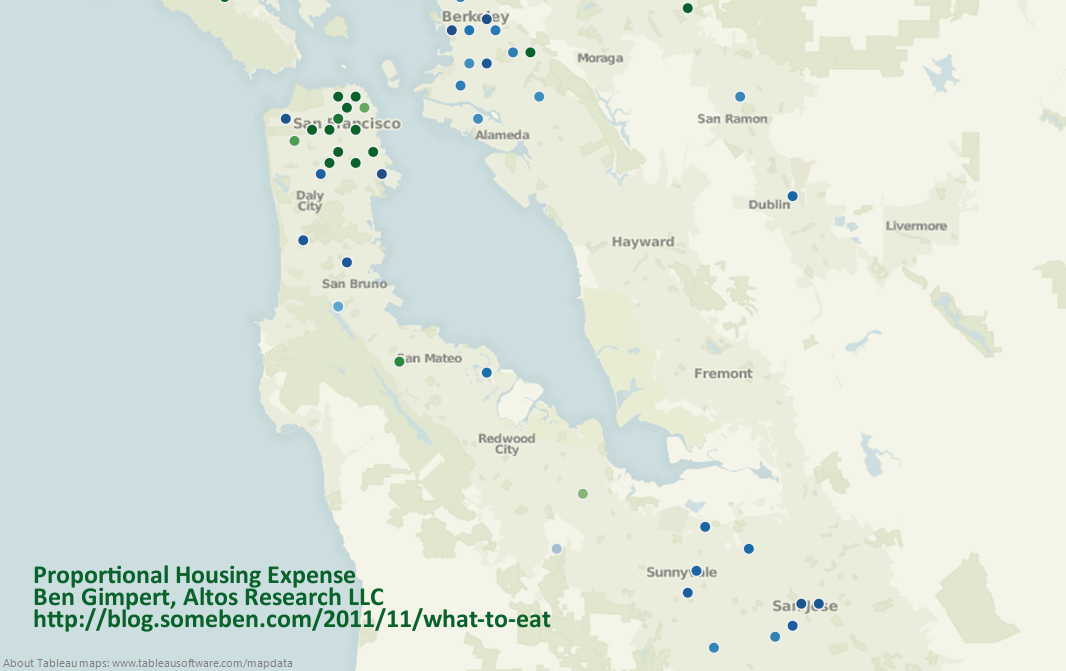
Bay Area Housing Proportional Housing Expense

The data shows that people living in the city of San Francisco spend a much larger proportion of their income on housing than Oaklanders or those in San Jose. If we assume that the real estate market is somewhat efficient, then those who choose to live in certain neighborhoods forgo savings and disposable income. Why is it that housing expenses for living in San Francisco are so much higher than San Jose, even when we control for income disparity?

The Real Estate Menu
Like a proper hack economist, I am going to gloss over the obvious driving factors of proportionally expensive housing, such as poor labor mobility, lack of job opportunities, and a history of minority disenfranchisement. I am a chef by training — culinary arts degree from CHIC, the Le Cordon Bleu school in Chicago — and remain fascinated by the hospitality industry. So instead of diving into big social problems, I focused on something flippant and easy to measure: Where people go out to eat, across areas with different levels of proportional housing expense.

I analyzed the menus of a random selection of 5,400 sit-down and so-called “fast casual” restaurants across the United States. This menu population is hopefully large and diverse enough to represent dining out in general, though it is obviously biased toward those restaurants with the money and gumption to post their menus online. However there is not a disproportionate number of national chain restaurants, since even the most common restaurant, T.G.I. Friday’s, is only about 2.5% of the population:
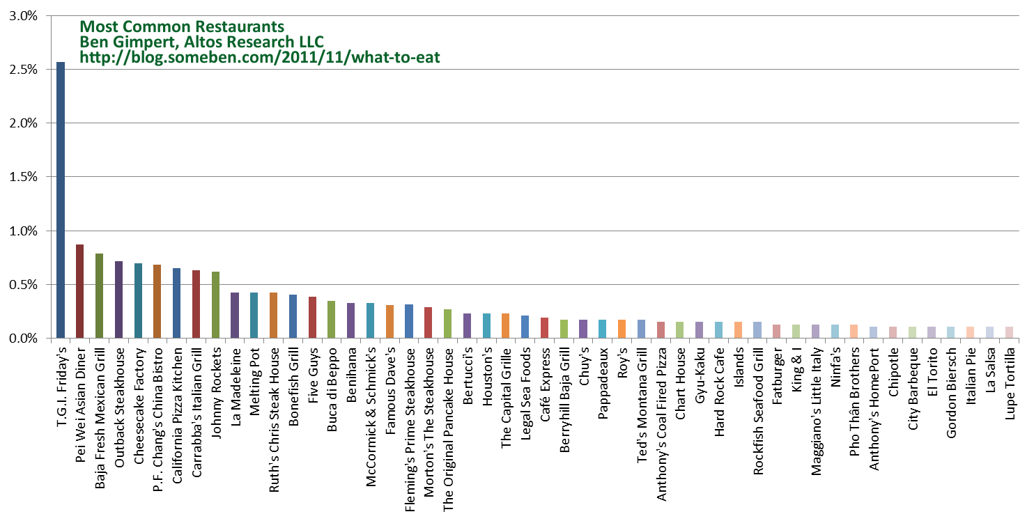
Restaurant Histogram

Menu Words
The next step in my analysis was counting the common words and phrases across the menus. Here are the top fifty:

1. sauce, 2. chicken, 3. cheese, 4. salad, 5. grilled, 6. served, 7. fresh, 8. tomato, 9. shrimp, 10. roasted, 11. served-with, 12. garlic, 13. cream, 14. red, 15. fried, 16. onions, 17. tomatoes, 18. beef, 19. rice, 20. onion, 21. bacon, 22. topped, 23. mushrooms, 24. topped-with, 25. steak, 26. vinaigrette, 27. spinach, 28. lettuce, 29. pork, 30. green, 31. potatoes, 32. spicy, 33. white, 34. salmon, 35. in-a, 36. soup, 37. peppers, 38. mozzarella, 39. lemon, 40. sweet, 41. with-a, 42. menu, 43. beans, 44. dressing, 45. fries, 46. tuna, 47. black, 48. greens, 49. chocolate, 50. basil

Pervasive ingredients like “chicken” turn up, as do common preparation and plating terms like “sauce” and “topped-with”. Perhaps my next project will be looking at how this list changes over time. For example, words like “fried” were taboo in the 90’s, but more common during this post-9/11 renaissance of honest comfort food. Now-a-days chicken can be “fried” again, not necessarily “crispy” or “crunchy”.

A Tasty Model
Next I trained a statistical model using the menu words and phrases as independent variables. My dependent variable was the proportional housing expense in the restaurant’s zipcode. The model was not meant to be predictive per se, but instead to identify the characteristics of restaurant menus in more desirable areas. The model covers over five thousand restaurants, so menu idiosyncrasy and anecdote should average out. The algorithm used was our bespoke version of least-angle regression with the lasso modification. It trains well on even hundreds of independent variables, and highlights which are most informative. In this case, which of our many menu words and phrases are correlated with proportional housing expense?

Why Clams are Bourgeois

The twenty menu words and phrases most correlated with low proportional housing expense (the bluer dots) areas:

1. tortilla, 2. cream-sauce, 3. red-onion, 4. thai, 5. your-choice, 6. jumbo, 7. crisp, 8. sauce-and, 9. salads, 10. oz, 11. italian, 12. crusted, 13. stuffed, 14. marinara, 15. broccoli, 16. egg, 17. scallops, 18. roast, 19. lemon, 20. bean

Several of these words of phrases are associated with ethnic cuisines (i.e. “thai” and “tortilla”), and others emphasize portion size (i.e. “jumbo” and “oz” for ounce). Restaurants in high proportional housing expense areas (greener dots) tend to include the following words and phrases on their menus:

1. clams, 2. con, 3. organic, 4. mango, 5. tofu, 6. spices, 7. eggplant, 8. tomato-sauce, 9. cooked, 10. artichoke, 11. eggs, 12. toast, 13. roll, 14. day, 15. french-fries, 16. duck, 17. seasonal, 18. oil, 19. steamed, 20. lunch, 21. chips, 22. salsa, 23. baby, 24. arugula, 25. red, 26. braised, 27. grilled, 28. chocolate, 29. avocado, 30. dressing

These words reflect healthier or more expensive food preparation (i.e. “grilled” or “steamed”), as well as more exotic ingredients (i.e. “mango” and “clams”). Also, seasonal and organic menus are associated with low proportional housing expense. The word “con” turns up as a counter-example for Latin American cuisine, as in “con huevos” or “chili con queso”.

Food Crystal Ball
This sort of model for restaurant menus could also be used for forecasting, to statistically predict the sort of food that will be more successful in a particular neighborhood. This predictive power would be bolstered by the fact that the population of menus has a survivorship bias, because failed or struggling restaurants are less likely to post their menus online.

This confirms my suspicion that housing expense is counter-intuitive when it comes to dining out. People who spend more of their income on housing in order to live in a desirable location have less disposable income, but these are the people who pay more for exotic ingredients and more expensive food preparation. Maybe these folks can’t afford to eat in their own neighborhood?

Sarah Palin Email Word Cloud

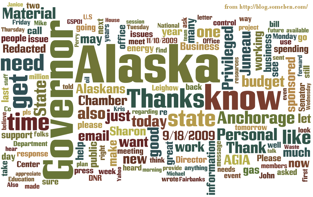
After three years of legal wrangling, the diligent folks at Mother Jones released another set of Sarah Palin’s emails on Friday. There are plenty of subtleties to the story. Should a personal Yahoo! email account be used for government work? And why the frustrating digital / analog loop of printing emails to be scanned at the other end, like a fax machine?

For my own snickering, I spent a couple hours over the weekend downloading the email PDF’s, converting them to text, and then parsing out the choice “holy moly’s” and tender bits about Track in the army. Here is a word cloud of the former governor’s emails, via the amazing Wordle project.

Sarah Palin's Email Word Cloud

Sour Grapes: Seven Reasons Why “That” Twitter Prediction Model is Cooked

The financial press has been buzzing about the results of an academic paper published by researchers from Indiana University-Bloomington and Derwent Capital, a hedge fund in the United Kingdom.

The model described in the paper is seriously faulted for a number of reasons:

1. Picking the Right Data
They chose a very short bear trending period, from February to the end of 2008. This results in a very small data set, “a time series of 64 days” as described in a buried footnote. You could have made almost 20% return over the same period by just shorting the “DIA” Dow Jones ETF, without any interesting prediction model!

There is also ambiguity about the holding period of trades. Does their model predict the Dow Jones on the subsequent trading day? In this case, 64 points seems too small a sample set for almost a year of training data. Or do they hold for a “random period of 20 days”, in which case their training data windows overlap and may mean double-counting. We can infer from the mean absolute errors reported in Table III that the holding period is a single trading day.

2. Massaging the Data They Did Pick
They exclude “exceptional” sub-periods from the sample, around the Thanksgiving holiday and the U.S. presidential election. This has no economic justification, since any predictive information from tweets should persist over these outlier periods.

3. What is Accuracy, Really?
The press claims the model is “87.6%” accurate, but this is only in predicting the direction of the stock index and not the magnitude. Trading correct directional signals that predict small magnitude moves can actually be a losing strategy due to transaction costs and the bid/ask spread.

They compare with “3.4%” likelihood by pure chance. This assumes there is no memory in the stock market, that market participants ignore the past when making decisions. This also contradicts their sliding window approach to formatting the training data, used throughout the paper.

The lowest mean absolute error in predictions is 1.83%, given their optimal combination of independent variables. The standard deviation of one day returns in the DIA ETF was 2.51% over the same period, which means their model is not all that much better than chance.

The authors also do not report any risk adjusted measure of return. Any informational advantage from a statistical model is worthless if the resulting trades are extremely volatile. The authors should have referenced the finance and microeconomics literature, and reported Sharpe or Sortino ratios.

4. Backtests & Out-of-sample Testing
Instead of conducting an out-of-sample backtest or simulation, the best practice when validating an un-traded model, they pick the perfect “test period because it was characterized by stabilization of DJIA values after considerable volatility in previous months and the absence of any unusual or significant socio-cultural events”.

5. Index Values, Not Prices
They use closing values of the Dow Jones Industrial Average, which are not tradable prices. You cannot necessarily buy or sell at these prices since this is a mathematical index, not a potential real trade. Tracking errors between a tradable security and the index will not necessarily cancel out because of market inefficiencies, transaction costs, or the bid/ask spread. This is especially the case during the 2008 bear trend. They should have used historic bid/ask prices of a Dow Jones tracking fund or ETF.

6. Causes & Effects
Granger Causality makes an assumption that the effects being observed are so-called covariance stationary. Covariance stationary processes have constant variance (jitter) and mean (average value) across time, which is almost precisely wrong for market prices. The authors do not indicate if they correct for this assumption through careful window or panel construction.

7. Neural Parameters
The authors do not present arguments for their particular choice of “predefined” training parameters. This is especially dangerous with such a short history of training data, and a modeling technique like neural networks, which is prone to high variance (over-fitting).